10 Key Data Preparation Steps for Building Accurate AI Models
Snehal Joshi
June 2nd, 202620 min read
AI models trained using corrupted, unrepresentative, or leakage-contaminated data fails in production. Your model learns the noise and the duplicates in your training set and generalizes those errors to live inference. Adhering to data preparation steps directly gates the quality of training data to prevent this failure.
Imagine your AI model showed 96% accuracy in the training phase but failed miserably in production within weeks. Hyperparameters were tuned perfectly and architecture was really sound. So then why did it fail? The problem is the use of biased, unrepresentative, and contaminated data in the training loop. And this has not happened with you only. Instead, it is the most common and preventable failure in machine learning projects.
Data preparation is exactly what sets your AI model for success or failure. Anaconda’s State of Data Science surveyed 3,493 practitioners across 133 countries to conclude that data scientists spend an average of 37.75% on data preparation and cleansing. This is not their core task, but to ensure the model succeeds they have to do it.
Why data preparation is important for building accurate AI models
Your AI model learns the right patterns only if it is fed clean, well-structured, representative data. Feed it noisy, incomplete, or biased data and it will not only learn wrong things but will carry those errors into every prediction it makes during production. This makes data preparation important for developing successful AI models.
Other reasons that make data preparation important for developing AI models include, your model cannot correct for label errors used to train it, your model is not capable of generalizing to demographics that were not included in the training datasets, neither can your model compensate for leaked feature information across the train-test boundaries.
All of these are not model problems. These all are data problems and they should be addressed upstream before initiating the training process.
Attributes that operate within a ceiling set by data quality include model architecture, hyperparameter tuning, and inference optimization. Disciplined data preparation approach will help you raise the ceiling if you are looking to make downstream ML decisions more reliable.
Operational challenges enterprises face during ML data preparation
Most enterprise ML pipelines don’t fail because of weak models. They failed because the data infrastructure behind them was not built to support production-scale preparation.
Data silos: Siloed data across divisions, CRM systems, ERP platforms, data lakes, third-party feeds and many more, exist in their own schema, access controls, and update frequency. Converting all of them into a unified, model-ready training dataset needs robust integration that we underestimate.
Annotation at scale: This compounds the problem. Labeling volumes of images, documents or audio files precisely requires agile and structured workflows, expert and experienced annotators and multi-level quality checks. In absence of any one of these, the label quality will drop substantially in spite of increased throughput.
Multilingual and multimodal datasets: These diverse datasets add up to the complexities. Imagine if a single data pipeline wants you to simultaneously handle English contracts, Mandarin customer records, scanned invoices, and sensor logs.
Version control of datasets: This is an afterthought in most of the pipelines, but it is ineffective. It will not allow you to reproduce a model or trace a performance regression to its source.
Compliance requirements: GDPR, HIPAA, SOC 2 define how you store, process and share data; and adds governance overhead at every stage.
10 key data preparation steps for building accurate AI models
The ten data preparation steps for machine learning encompasses ten stages. Starting right from defining scope of data problem to auditing data sources, and cleaning, validation, feature engineering, and annotation, to versioning and pipeline governance.
Each of the ten steps in a sequence below are backed by tools and techniques that determine whether your model will generalize or not.
Step 1 – Define the problem scope and data requirements
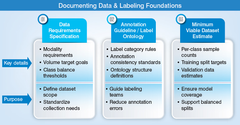
Before your team starts collecting or cleaning any data, you should lock the task definition. Their first step should be to define the problem of scope and identify data requirements. They might come up with the question as to why data requirements must precede data collection.
And the answer to the question is that classification, regression, object detection, named entity recognition, time-series forecasting and several others will inflict various requirements on data modality, volume, label granularity, and acceptable ground truth ambiguity.
Defining the problem scope and data requirements will help you come up with three documents:
No AI teams can afford to skip this step. Doing so may lead your teams to realize that bounding box annotations required semantic segmentation masks, or the regression target should have been treated as ordinal classification. At the same time, you cannot afford to rebuild a labeling schema once the annotation is complete proves to be a really expensive error in an ML pipeline.
However, if the requirements are defined and locked, it will help in evaluating candidate data sources against the specifications locked. Your teams will no longer have to adjust specifications to match whatever data is available.
Step 2 – Data collection and source auditing
Data sources for ML projects include proprietary databases and open repositories like Hugging Face Hub, UCI ML Repository, Kaggle. Also, web-scraped corpora and synthetic generation pipelines like diffusion models, & GANs are also important.
And yes, don’t forget to add third-party data annotation service providers or third party data annotation partners to the list. It might look lucrative, but each of them carries distinct risk profiles, warranting source auditing.
At this stage, the source audit will evaluate three things:
Selection bias to see if the source systematically underrepresents subgroups that may appear at inference
Temporal drift to check if data was collected under conditions that no longer match your deployment context
Licensing constraints to verify CC-BY vs. commercial use restrictions, data residency requirements, etc.
Three data collection pitfalls that surface later when your AI model fails
Convenience sampling: It will underrepresent edge cases. You may train your fraud detection model on flagged transactions from a single region. But now they will underperform on cross-regional fraud patterns.
Mixing data: You may have collected data under different sensor configurations or annotation schemas, and now your Ai teams are mixing it without versioning the schema change as a dataset boundary.
Absence of metadata: Avoiding adding metadata like timestamps, source device IDs, collection geography and other such attributes, which you need later for stratified splitting and drift monitoring, will lead to failure.
Adhering to this step will not give you a dataset. But it promises you that all the data you collect will be sourced and audited with authentic documentation. This matters the most when you are stuck and want to trace a model’s performance regression to a specific data intake batch.
Step 3 – Exploratory data analysis (EDA) and data profiling
Up till now we defined the scope of problem, basis which we also decided which and how to evaluate data sources for bias, coverage, and licensing. So, it’s time we discuss data profiling and exploratory data analysis. Yes, the distributions, correlations, and outliers that are the determinant to which data cleansing strategy should select.
The very first thing that we need accept is that data profiling and exploratory data analysis – EDA are meant for two different purposes, so do not conflate.
You can use data profiling for automated schema and statistical summarization of null matrices, dtype inference, value frequency histograms, cardinality counts. Using tools like ydata-profiling, Sweetviz, and D-Tale will help you generate these HTML reports in less than minutes.
At the same time, exploratory data analysis – EDA, is analyst-driven investigation. It mainly supports you to determine cleaning and transformation activities like:
Missingness pattern classification
Class imbalance ratios
Feature correlation matrices – Use Pearson for continuous and Cramer’s V for categorical
Outlier distributions – Use Z-score and IQR for univariate and Isolation Forest for multivariate
Missingness pattern classification is a fundamental concept in data analysis. Missing data is rarely random. Missing data more than often carries its own signal which is systematically related to unobserved factors. Ignoring these signals will result in biased, inaccurate, or misleading results.
Missing data, though a negative aspect, is very critical to know everything about it. We can classify the missing data in three categories:
Missing Data Type
Definition Highlights
Example Scenario
Key Implication
MCAR: Missing Completely at Random
Fully random missingness
No variable relationship
Independent missing patterns
Lost survey forms
Random questionnaire loss
Unbiased analysis results
Reduced statistical power
MAR: Missing at Random
Explained by variables
Observed data dependency
Pattern-based missingness
Gender-linked nonresponse
Income reporting gaps
Potential analysis bias
Multiple imputation useful
MNAR: Missing Not at Random
Self-related missingness
Unobserved value dependency
Reason-driven data absence
High-income nonreporting
Sensitive response avoidance
Significant bias risk
Difficult correction process
Why missingness pattern classification is important for data profiling?
Understanding the “Why” behind missing data is extremely important for data profiling and EDA activities.
Listwise Deletion (Dropping Missing Values): You cannot just remove rows that have missing data, aka, listwise deletion. It works only for MCAR. But for MAR or MNAR, it will remove important and non-representative data while will introduce bias also.
Imputation Method: Do not make the mistake of replacing missing values with mean, it will surely create biased, and false data. The better way to do it is to include multiple imputation or use models that account for the missingness.
Systematic Patterns: Missing data is a signal that there are errors like a sensor wearing out over time or specific behaviors.
Your Data preparation teams can use Apache Spark and BigQuery ML to expose equivalent profiling functions at distributed scale when working with too large datasets. They can also use Google’s PAIR Facets tool for interactive slicing of training data distributions across categorical dimensions. It will help them in identifying subgroup representation gaps before cleaning.
Step 4 – Data cleaning for missing values, de-duplication, and handling noise
Till now we learnt and read about what to do, and so now we will see how to choose the right strategy for missing values, noise, and duplicates.
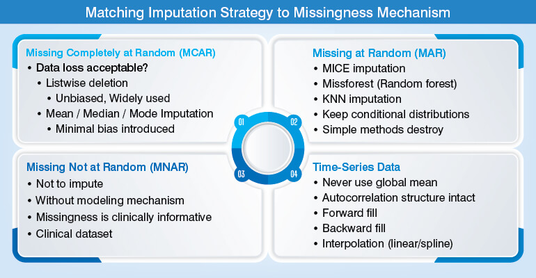
Your data professionals can execute and implement all the EDA findings in this very crucial step of data cleansing. The problems of missing values, duplicate records, and noisy labels or features should be handled distinctly. For imputing missing values match the strategy to the mechanism.
For values Missing Completely at Random – MCAR: If your team is fine with data loss, listwise deletion is unbiased and hence widely used. Using mean/median/mode imputation may introduce minimal bias to the dataset.
For Missing at Random – MAR: You can use Multiple Imputation by Chained Equations- MICE, random forest-based – MissForest, or KNN imputation. These techniques keep conditional distributions intact, which simpler methods destroy.
For Missing Not at Random – MNAR: Missingness pattern is a binary feature. Advise is to not to impute without modeling the mechanism. For example, in a clinical dataset, a missing lab value is itself clinically informative.
For Time-series: It is suggested to never use global mean imputation. Instead you should resort to forward fill, backward fill, or interpolation (linear or spline) to keep the autocorrelation structure intact.
Why exact match is not enough for deduplication?
You can use hash-based exact deduplication to handle identical records. And for near-duplicate removal you can use fuzzy methods like MinHash LSH for text corpora, Levenshtein distance for short strings, and of course perceptual hashing for images. If you inflate near-duplicates in the training set, it will eventually improve the training metrics and degrade generalization. Do not confuse evaluation gain with model improvement.
Why label noise is a ceiling problem?
Label noise is not an edge case. On average 3.3% of errors were identified when 10 of the most commonly used computer vision, natural language and audio datasets were inspected. Also, 2916 label errors comprise 6% of the ImageNet validation set. You can go ahead and use confident learning algorithms to identify putative label errors; and then validate them using human-in-the-loop approach.
According to Journal of Engineering and Artificial Intelligence 60% asymmetric label noise on CIFAR-10, ResNet-18 test accuracy dropped to 38.7% with Expected Calibration Error exceeding 35%.
Experienced and expert data preparation service providers leverage confident learning to algorithmically identify likely label errors at scale. For subjective labeling tasks they deploy inter-annotator agreement scoring. For categorical labels they use Cohen’s kappa, and for ordinal they use Krippendorff’s alpha. It provides a quality floor before any model could see the data.
Once done with data cleansing, validate the data against schema expectations before you move it to transformation. Data cleaning and data transformation are two different data pipeline stages.
Step 5 – Data validation and schema enforcement
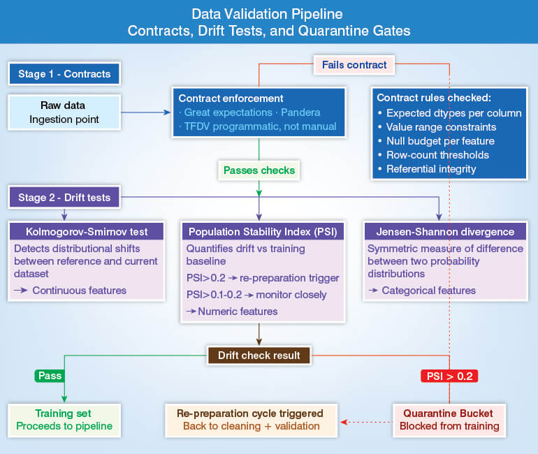
Data validation and schema enforcement; both these foundational techniques take care of data quality, consistency, and reliability across modern data systems. Though used together they serve individual roles in a data pipeline.
The process of data validation will operationalize your quality expectations as a code. As you know, manual spot checks are not scalable and also, they do not provide audit trails.
Operational implication of data validation and schema enforcement is very simple. Data that fails validation checks is routed to quarantine bucket. It should not reach the training dataset. This is the gate that prevents a corrupt batch of data from silently degrading a model which was working fine before it entered the workflow.
The next step, after data validation, is restructuring it into numeric representations which ML algorithms can consume. That’s where feature engineering and transformation enters the picture.
Step 6 – Feature engineering and transformation
Feature engineering and transformation is all about scaling, categorical encoding, and building features without leaking information across splits. The process of converting validated data into numeric presentations is also critical because the choices made here will directly affect both; your model’s accuracy and the validity of your evaluation metrics.
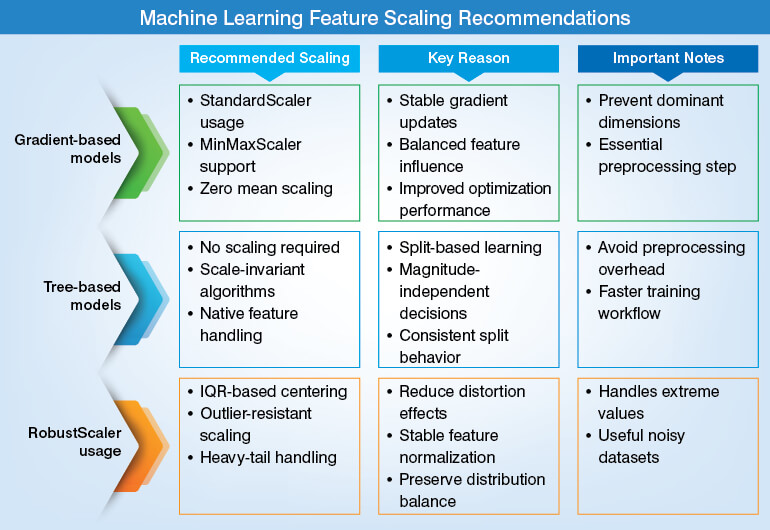
Which models care in feature scaling?
Feature scaling is a critical pre-processing step for ML models that calculate distances between data points or use gradient-based optimization. If you don’t scale features with different ranges (e.g., age vs. salary) it will make your model prioritize variables with larger magnitudes, and make it biased, inaccurate, and slow-to-converge.
How to match cardinality to method for categorical encoding?
In order to prevent overfitting, manage memory, and improve model accuracy matching the correct categorical encoding method to cardinality – number of unique categories, of a feature is mandatory. High-cardinality features can create standard methods like One-Hot Encoding for creating too many dimensions, while low-cardinality features may not capture complex relationships even while using advanced methods.
Category Type
Recommended Encoding
Key Characteristics
Important Considerations
Low-Cardinality Nominals
One-hot encoding
Binary column creation
Separate category fields
Fewer unique values
Independent category handling
Clear feature separation
Suitable small categories
Easy model interpretation
High-Cardinality Nominals
Target encoding usage
Leave-one-out encoding
Fold-based fitting
Many unique values
Compact feature representation
Leakage-sensitive processing
Prevent target leakage
Use cross-validation folds
Ordinal Categories
Ordinal encoding method
Rank-preserving transformation
Ordered category mapping
Natural value hierarchy
Sequential category relationship
Structured category levels
Maintain ranking order
Preserve relational meaning
How to prevent data leakage during feature engineering?
Data leakage is normal when all the available information at the time of interference is encoded in training features. Also, it can happen when a transformation fit on the full dataset is applied without splitting it. Both situations inflate evaluation metrics while guaranteeing production underperformance.
The mechanical solution to prevent data leakage during feature engineering is to wrap all transformations in a scikit-learn Pipeline or FeatureUnion. Ensure you fit the pipeline on the training split only. Start by applying transform only, not fit; on validation and test. Feature that encodes information from after the prediction is a leakage vector and must be dropped immediately.
Step 7 – Dimensionality reduction and feature selection
Engineered features will amplify signals, but what will you do with datasets that contain hundreds of them. To prevent the mishap of dimensionality, dimensionality reduction and feature selection becomes mandatory.
There are three selection paradigms; filter, wrapper, and embedded methods, and you should know when to use which, as each of them optimizes for a different trade-off.
Feature Selection Method
Common Techniques
Key Advantages
Important Limitations
Filter Methods
Variance threshold filtering
Mutual information scoring
ANOVA F-statistic
Chi-squared testing
Model-agnostic approach
Computationally inexpensive
Fast feature pruning
Lower selection fidelity
Limited interaction awareness
Wrapper Methods
Recursive feature elimination
Sequential forward selection
Sequential backward selection
Higher selection accuracy
Subset performance evaluation
Better feature combinations
Computationally expensive
Repeated model fitting
Limited large datasets
Embedded Methods
L1 regularization usage
Lasso feature selection
Tree importance scores
SHAP value analysis
Integrated training process
Production pipeline friendly
No extra data loops
Model-dependent selection
Interpretation complexity possible
How to reduce dimensionality for unstructured data?
To reduce dimensionality for unstructured data like text, images and audio; transform high-dimensional raw data into lower-dimensional representations. Retain the essential information while doing this. Key techniques used to reduce dimensionality in unstructured data includes use of deep learning models (Autoencoders, CNNs) for feature extraction, embedding techniques (BERT, Word2Vec for text), and algorithms like PCA, t-SNE, or UMAP to compress high-dimensional vectors.
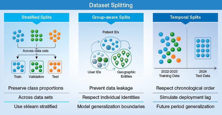
Step 8 – Dataset splitting, stratification, and class imbalance handling
With a compact, informative feature set, the next decision that you would be making is how to split and sample the data; a stage where class imbalance should be addressed directly.
For an independent, identically distributed tabular dataset with balanced classes, you can go ahead and use the random 80/20 train-test split. However, chances that real-world ML datasets meet those conditions is very less.
Data analytics company serving government agencies partnered with Hitech BPO to prepare voluminous training data to be fed to their machine learning project. The final solution predicted traffic issues, prevented accidents, improved road planning, and assisted in civil engineering projects.
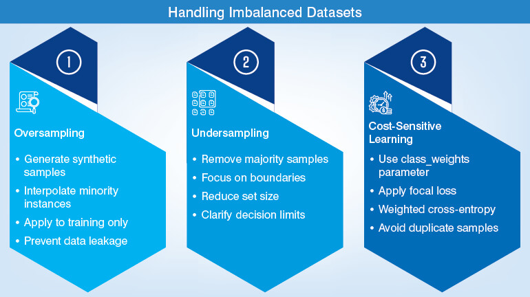
How to handle class imbalance without inflating your metrics?
Class imbalance causes standard accuracy which is misleading. A classifier predicts the majority class with 99% accuracy, 100% of the time on a dataset with 1% positive class prevalence. You can use Precision-recall AUC, Matthews Correlation Coefficient (MCC), and macro-average F1 which are considered to be the correct metrics for imbalanced problems.
Now that your training dataset is structured correctly check out on what it lacks for supervised learning. Yes, you guessed it right. It is reliable ground truth which makes accurate data annotation a necessity.
Step 9 – Data annotation, labeling quality, and ground truth validation
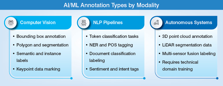
For supervised learning, high-quality annotation of your training datasets is the hard ceiling on model performance. No right or wrong choice of architecture, no hyperparameter tuning, and no augmentation strategy would help you recover accuracy lost due to systematic label errors. This is why inter-annotator agreement, and adjudication protocols belong in your pipeline specs.
It helps you to establish the ceiling principle where “if a model is trained on noisy labels, it should not generalize beyond the accuracy of those labels”. So, this way, a 5% label error rate should set the practical upper bound on test accuracy.
Annotation types vary by modality, and all of these demand annotators with domain-specific technical training.
A Swiss food waste management company partnered with Hitech BPO for accurate and timely training data preparation. It enhanced their ML models’ ability to analyze visual data effectively, supporting their mission to combat food waste in hotels and restaurants.
How to have a quality control process that catches annotator drift before it reaches training?
ISO 27001-certified annotation workflows: Start with this as it is a mandate for annotating data of regulated domains including healthcare imaging, financial document processing, autonomous vehicle data. The certifications will ensure designated access, audit trails and data handling protocols meet your enterprise data security requirements.
Multi-annotator consensus with adjudication: Once the workflow is set, it’s time to chart the guidelines. So majority vote for clear-cut cases. Expert tie-breaking for unclear samples and use of STAPLE algorithm for probabilistic label fusion across your team of data annotators.
Inter-annotator agreement (IAA) measurement: Not because we as a leading data annotation service provider use it, but all AI and ML companies leverage Cohen’s kappa for binary and multi-class categorical labels. They also use Krippendorff’s alpha for ordinal or interval scales and rely heavily on Intersection-over-Union (IoU) for bounding box quality assessment.
Embedded gold-standard tasks: Injecting a sample of pre-verified known-answer items into each annotation batch. This will help you have a continuous quality signal about annotator accuracy on these tasks. It will also identify and flag individual annotators whose performance is going downhill.
Having a fully annotated and validated training dataset is not the end of story. It will still need infrastructure to ensure that it remains reproduceable and auditable across model iterations. And to address it you need data versioning and pipeline governance.
Step 10 – Data versioning, lineage tracking, and pipeline governance
Do you know that the same code on different dataset versions produces different models. Yes, that’s true. Dataset versioning is a prerequisite for model reproducibility. But, if you version the first two without versioning the third, it will make model reproducibility nearly impossible. The same code on v1 vs. v2 of a training set produces different models. Most AI and ML companies consider dataset versioning as an optional activity, instead they should consider it to be a MLOps hygiene practice, which is warranted for debugging production regressions.
To keep a track of datasets without duplicating large binary files in version control you can take snapshots by integrating Data Version Control – DVC with GIT. Every training run will tag a dataset version hash. It empowers you to reproduce the exact training set that produced it, just in case any of your model’s performance degrades during production.
Why use data lineage to trace what produced each dataset version?
Using data lineage is suggested as it records which raw sources, transformation steps and annotation runs produced each version of any dataset. Apache Atlas, MLflow, Weights & Biases Artifacts are the tools that implement OpenLineage metadata collection making the activity traceable and queryable. Plus, nowadays, for some regulated industries, lineage documentation has become a compliance item and not just a data engineering convenience.
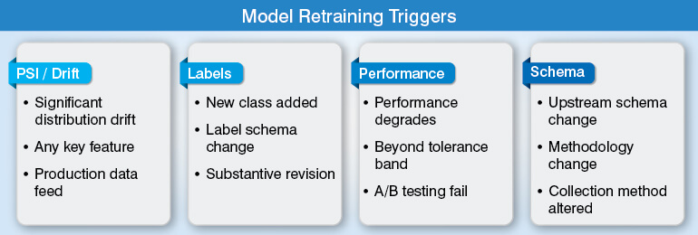
When to trigger a full re-preparation cycle?
Here, we have simplified the criteria into clear and concise bullet points for better understanding of one and all. It highlights indicators like significant distribution drift, revised label schemas, performance degradation, and of course upstream schema changes as well.
Which are compliance-specific governance requirements in preparing data for AI models?
How training data is stored, accessed, and destroyed have separate requirements when it comes to compliance to governance norms.
Documented PII scrubbing procedures with audit trails is the primary requirement of GDPR-compliant preprocessing.
Safe Harbor (removal of 18 specific identifiers) or Expert Determination (statistical demonstration of re-identification risk below threshold) is required for HIPAA de-identification.
AI and ML companies should ensure to build these into the pipeline specification, and not as post-hoc overlays.
Conclusion – Data preparation makes or breaks the accuracy of your AI model
None of the 10 data preparation steps that we talked about in the article are independent tasks. They are a sequential pipeline, where the output of the previous step becomes the input of the next step. Cut down or skip any of the step, and the errors will propagate forward.
For AI teams working on large-scale, multi-modal, or regulated ML datasets, adhering to all 10 steps will require dedicated tools and technology, annotator infrastructure and a robust QC process that internal teams are rarely staffed with to manage and maintain end-to-end data preparation process.
FAQs
Data preparation is important for building accurate AI models because every AI model learns directly from its training data. If the training dataset is filled with errors, bias, or missing values, the model will learn those flaws and carry it to production. Data preparation fixes these errors before the training begins and sets quality for architecture choices, hyperparameter tuning, and inference optimization.
There are sever challenges enterprises face during ML data preparation. First is data scattered across CRM platforms, ERP tools, and data lakes, each of them with diverse schemas and access rules. Second is annotating Multilingual and multimodal datasets in a separate pipeline at scale. Then there is a drop in labeling quality in absence of structured quality check workflow. Compliance to GDPR and HIPAA adds overhead.
Exploratory data analysis (EDA) improve AI model accuracy by highlighting problems like skewed class distributions, correlated features, multivariate outliers, and missing data patterns. It also helps in identifying MCAR, MAR, or MNAR missingness and also the imputation strategy. Not using EDA is as good as making preprocessing decisions based on guesswork.
dataset splitting and handling class imbalance are important in AI because the first one determines whether your evaluation metrics reflect real deployment conditions, whereas the later if unaddressed, causes models to favour the majority class. This makes standard accuracy misleading.
Data validation and schema enforcement play an important role in AI pipelines. The first one converts quality expectations into executable code. It also checks dtypes, value ranges, null budgets, and row counts automatically at the time of data ingestion. They also help in flagging incoming data that has shifted from the training baseline and sending it to a quarantine bucket instead of the training set.
Data versioning and lineage tracking are very critical for enterprise AI because same training code applied to two different dataset versions produces two different models and without versioning this difference becomes invisible and untraceable. Lineage tracking helps in recording which sources, transformations, and annotation runs created which dataset version.
Snehal Joshi spearheads the business process management vertical at Hitech BPO, an integrated data and digital solutions company. Over the last 20 years, he has successfully built and managed a diverse portfolio spanning more than 40 solutions across data processing management, research and analysis and image intelligence. Snehal drives innovation and digitalization across functions, empowering organizations to unlock and unleash the hidden potential of their data.
What’s next? Message us a brief description of your project. Our experts will review and get back to you within one business day with free consultation for successful implementation.
Disclaimer:
HitechDigital Solutions LLP and Hitech BPO will never ask for money or commission to offer jobs or projects. In the event you are contacted by any person with job offer in our companies, please reach out to us at info@hitechbpo.com
To provide the best experiences, we use technologies like cookies to store and/or access device information. Consenting to these technologies will allow us to process data such as browsing behavior or unique IDs on this site. Not consenting or withdrawing consent, may adversely affect certain features and functions.
Functional
Always active
The technical storage or access is strictly necessary for the legitimate purpose of enabling the use of a specific service explicitly requested by the subscriber or user, or for the sole purpose of carrying out the transmission of a communication over an electronic communications network.
Preferences
The technical storage or access is necessary for the legitimate purpose of storing preferences that are not requested by the subscriber or user.
Statistics
The technical storage or access that is used exclusively for statistical purposes.The technical storage or access that is used exclusively for anonymous statistical purposes. Without a subpoena, voluntary compliance on the part of your Internet Service Provider, or additional records from a third party, information stored or retrieved for this purpose alone cannot usually be used to identify you.
Marketing
The technical storage or access is required to create user profiles to send advertising, or to track the user on a website or across several websites for similar marketing purposes.